Do GPU-based Basic Linear Algebra Subprograms (BLAS) improve the performance of standard modeling techniques in R?
Introduction
The speed or run-time of models in R can be a critical factor, especially considering the size and complexity of modern datasets. The number of data points as well as the number of features can easily be in the millions. Even relatively trivial modeling procedures can consume a lot of time, which is critical both for optimization and update of models. An easy way to speed up computations is to use an optimized BLAS (Basic Linear Algebra Subprograms). Especially since R’s default BLAS is well regarded for its stability and portability, not necessarily its speed, this has potential. Alternative libraries are for example ATLAS and OpenBLAS which we will use below. Multiple blog-posts showed that they are able to improve the performance of linear algebra operations in R, especially those of the infamous R-benchmark-25.R.
With nvblas, nvidia offers a GPU-based BLAS-library, which it claims to be significantly faster than standard procedures. nvblas is part of the latest CUDA-implementations such as CUDA 9. According to nvidia, nvblas is able to speed up procedures such as the computation of the determinant of a 2500x2500 matrix by a factor of more than ten. However, most users from the data science sphere don’t use basic linear algebra operations directly - they usually use high-level-abstractions such as lm() or gam() for modeling.
With little effort we can swap the default BLAS to OpenBLAS and already get significant performance gains. And so we want to find out if nvblas can speed up computations just as easily! For this comparison we compare R’s default BLAS, the optimized libraries ATLAS and OpenBLAS (all of which are using CPUs only) with nvblas (which uses CPU and GPU).
Setup
We simulated data for three scenarios:
- Regression: We draw data for a fixed number of numerical and dummy variables (using a normal distribution with poison-distributed variance and mean 0 and a Bernoulli distribution with uniformly distributed probability, respectively) and calculate the target as a linear combination of the features, adding nonlinear interaction effects and a random error term. The following models are set up to solve this problem:
- Linear Regression: using glm(family = "gaussian") from stats
- Additive Regression: using bam(family = "gaussian") with max. 20 smoothed variables from mgcv
- Extreme Gradient Boosting: using xgb.train(nrounds = 30, tree_method = "hist") from xgboost, using a 75%-25% train-test-split
- Classification: We draw data in a similar fashion as with the regression example, but derive the binary outcome from the former dependent variable by splitting at the median of the outcome variable and adding an additional 5%-dropout. The following models are set up to solve this problem:
- Generalized linear Regression: using glm(family = "binomial") from stats
- Generalized additive Regression: using bam(family = "binomial") with max. 20 smoothed variables from mgcv
- Extreme Gradient Boosting: using xgb.train(nrounds = 30, tree_method = "hist") from xgboost, using a 75%-25% train-test-split
- Random Intercept: We draw data in a similar fashion as with the regression example, but adding an additional random intercept for random groups. The following models are set up to solve this problem:
- Linear Mixed Model: using lmer() from lme4
- Linear Mixed Model: using lme() from nlme
- Additive Mixed Model: using bam(family = "gaussian") with max. 20 smoothed variables and the bs parameter from mgcv
The particular pick of functions simply reflects which models and packages we currently use at INWT Statistics. So those are the most interesting ones for us to look at. When you have a thorough understanding of how these methods are implemented, you may, in part, anticipate some of the results. To execute the experiments, we used an AWS machine capable of both efficient CPU and GPU computations: p3.2xlarge with Machine Learning AMI containing the latest CUDA version. With this setup, it is relatively easy to change the BLAS library by configuring it via an environment variable:
env LD_PRELOAD=libnvblas.so Rscript code.R
To permanently switch the BLAS version, one can use update-alternatives:
sudo update-alternatives --config libblas.so.3gf
To check which BLAS and LAPACK-version a running R-console is using, do
ps aux | grep exec/R
to get the PID and then do:
lsof -p <PID> | grep 'blas\|lapack'
The xgboost-package plays a special role in our tests: additionally to change the BLAS-package to nvblas (the optimization done by xgboost does not improve much by using different blas-versions), one can change the optimization-algorithm to gpu-hist, if the package is installed correctly. This approach to the histogram tree growth method is optimized for GPUs and should outperform the cpu-version. This was done for our tests.
Results
The experiments were done for different sample sizes and numbers of categorical and numerical features. We show the results for a sample of 100,000 and 100 categorical as well as 100 numerical features. If you think this is small: we do not analyse images, videos or gene expression data; this is a somewhat realistic scenario in which performance becomes interesting and relevant for us.
The R-benchmark-25 needs 5.54 seconds using OpenBLAS, 11.21 seconds using ATLAS, 34.62 with the default BLAS and 7.78 - 8.08 seconds using nvblas, depending on OpenBLAS or ATLAS as fallback (which is specified in the nvblas.config). Even for R-benchmark-25, nvblas is not faster compared to OpenBLAS, however both run significantly faster than the default BLAS.
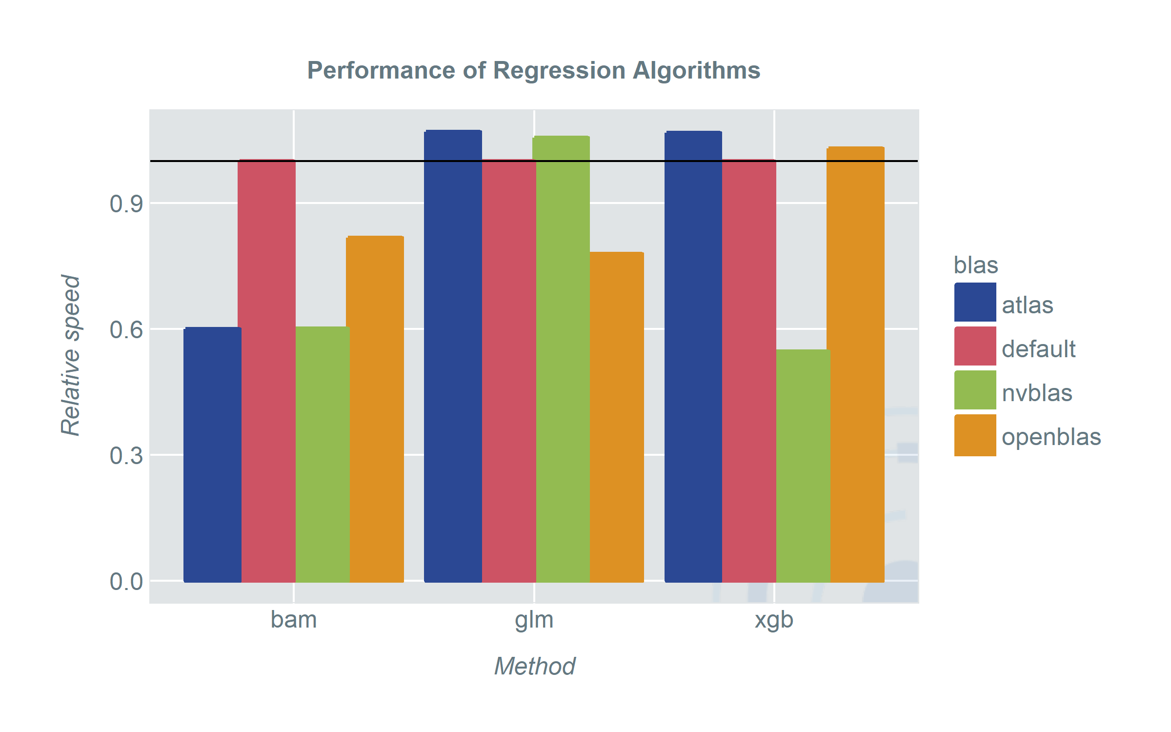
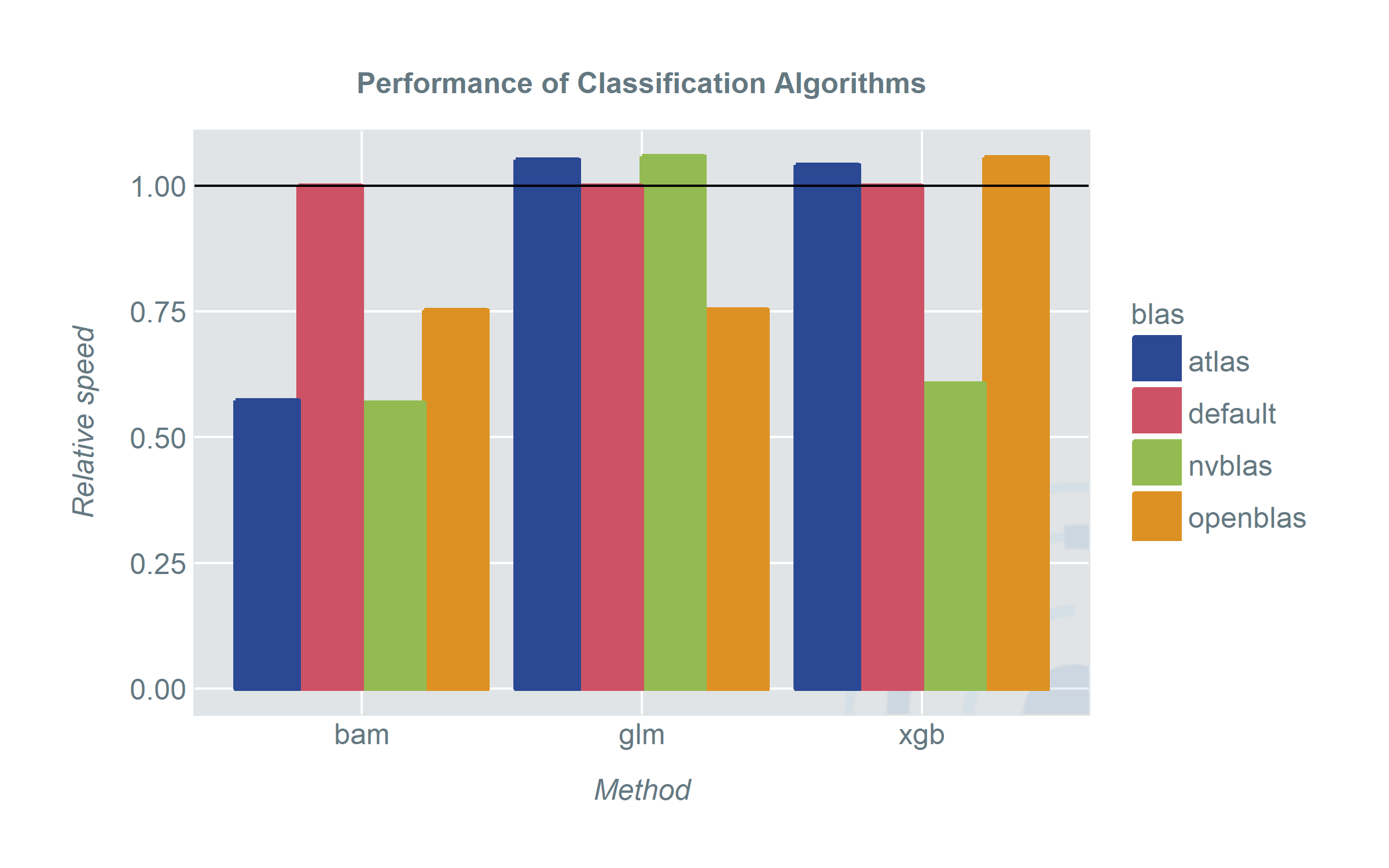
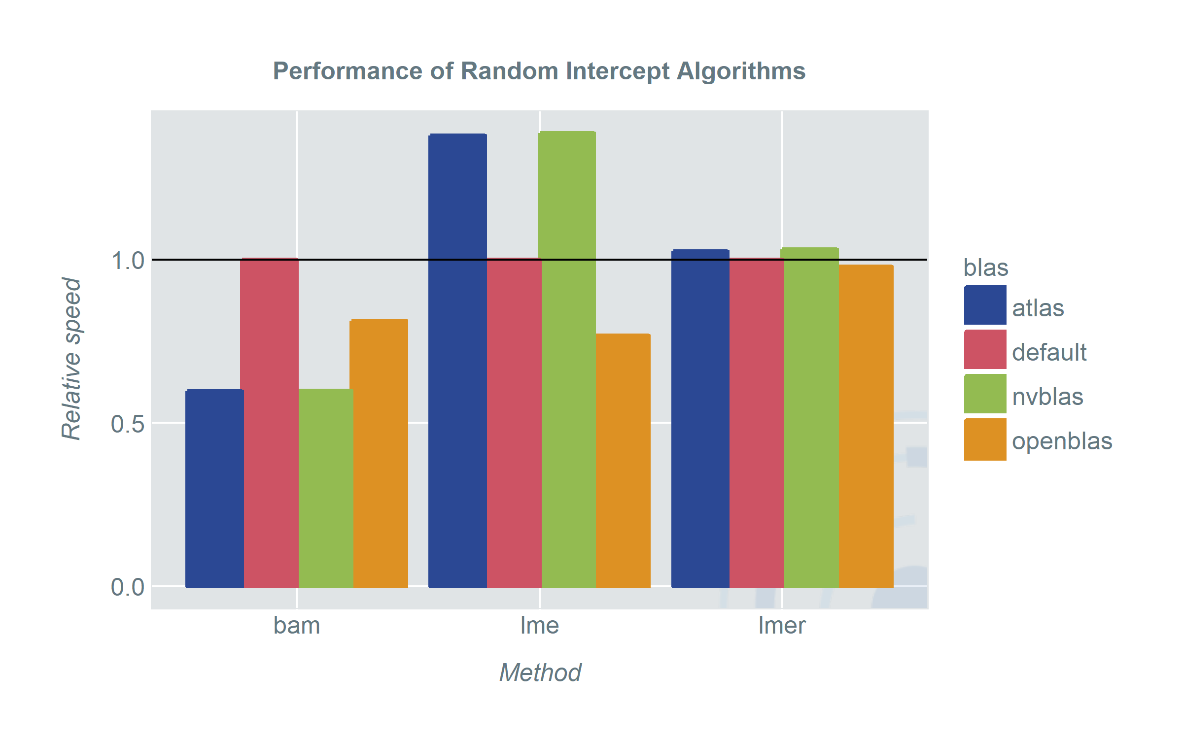
So how do the different BLAS-versions perform for high-level-functions in R? The plots show the speed of the methods using different BLAS-versions.
When we started out we were hoping for a clear winner and somehow we also found one. However depending on your pick of models and applications there are some unexpected results.
- No matter which BLAS library we used, bam picked it up and the run-time improved significantly. When we have a machine with sufficiently strong CPUs ATLAS is about as fast as using nvblas and a GPU. OpenBLAS still shows an improvement over the default BLAS. A good thing about bam is that it covers a wide range of model classes. Especially random intercept or generally random effect models (sadly) do not get a lot of attention in the machine learning era.
- xgboost gains from nvblas. This is not very surprising since it uses an optimized algorithm for GPUs. However, it does not gain anything from ATLAS or OpenBLAS.
- For the traditionalists: glm and lme will profit from OpenBLAS. Very surprising however is the performance loss when we used ATLAS and nvblas. Either we have a considerable overhead when using these libraries or the configuration is not as plug-and-play as we hoped for. In any case it is reason enough to praise OpenBLAS to speed up a lot of computations out of the box. Even when specialized models may gain more from other libraries.
- What is wrong with lmer: lme4 uses the RcppEigen package to replace the default BLAS library. For a lot of users this has the advantage that lmer will run fast without you doing anything. But since it is not using the default BLAS it will also not benefit from replacing it with ATLAS, OpenBLAS or nvblas. lmer and lme (OpenBLAS) have been comparable in run time in most of our tests. More pressing is the question which one implements the method you need.
We hoped to see that nvblas would easily outperform all other libraries. Of course it is not that simple. For statistical modeling, the libraries which have been tuned, optimized and debugged for decades are hard to beat. If you are looking for a plug-and-play speed improvement I would still vote for OpenBLAS.