Multi-Armed Bandits as an A/B Testing Solution

These days, most people are familiar with the concept of A/B testing. This is one of the most common ways to make advertising decisions, particularly in online marketing. In an A/B test, the customer base is divided into two or more groups, each of which is served a different version of whatever is being tested (such as a special offer, or the layout of an advertising campaign). At the end of the test, whichever variant was most successful is pursued for the customer base at large.

While this method is tried and true, there are some potential situations where it is less than ideal. For example, it is important for the integrity of the experiment that the results of A/B tests not be checked while the program is ongoing. But what if it turns out that one of the variants being tested is performing very poorly, or extremely well? That means that a portion of the customers aren’t going to be served optimally. 

If there is only one test, this opportunity cost is probably manageable, and worth the investment to discover the best possible variant. But in the event that many variants are being tested, a greater proportion of the customers will be served a suboptimal variant for a longer period of time, potentially resulting in significant costs.

In an ideal world, we’d want to be able to rule out the variants that are performing poorly very quickly, and only conduct a full A/B test on those variants that have promise or have proven to perform well. 

Multi-Armed Bandits as a Solution

Originally, slot machines were operated by pulling a lever, earning the name “one-armed bandits” given their penchant for cleaning out players’ bank accounts. The name “Multi-Armed Bandit” comes from the idea of playing multiple slot machines at once, each with a different unknown payoff rate. Our goal as the player would be to figure out which machine has the highest payoff rate, and play that machine more often than the others to maximize our rewards.

While it might seem like our goal would be to exclusively play the higher-payoff machine, unless we know for certain what the exact payoff rates are in advance (which we can’t in this scenario), we would want to continue playing the other machines for as long as it takes to be reasonably certain that we have selected the correct machine to prioritize.

This brings us to the concept of the exploration vs. exploitation trade-off (in layman’s terms, “learn or earn”). Basically, this is the trade-off between reward later (exploration) or now (exploitation).

An A/B test is purely exploratory: customers are randomly assigned to a variant, and the achievable payoff is simply the average payoff of all the variants (meaning that, by design, it will always be lower than the payoff of the strongest variant). There is no conscious exploitation of a higher-earning variant, which leads to “regret”: the difference between the optimal policy that we would choose if we knew the true payoff, and the action taken.

Bandit algorithms, on the other hand, seek to strike a balance between exploration and exploitation by exploring each variant sufficiently enough to identify the strongest variant, and then primarily exploiting the optimal action to maximize the total reward. The algorithm also continues to explore other possible variants to discover whether they become stronger in the future. The idea is to end up with a higher final reward (and thus, less regret), while still allowing the algorithm to continue gathering data on other variants.

Varieties of Multi-Armed Bandit Algorithms

There are many kinds of Bandit algorithms. Three of the most common - Epsilon Greedy, Upper Confidence Bounds, and Thompson Sampling - are briefly discussed here, to illustrate how these algorithms work in practice.

Epsilon Greedy

In the Epsilon Greedy (or ε-greedy) algorithm, after an initial number of purely exploratory trials, a random lever is pulled a fraction ε of the time. The rest of the time (1 - ε), the lever with the highest known payoff is pulled. For example, if we set ε to 0.10, 10% of the time the algorithm will explore random alternatives, and 90% of the time it will exploit the variant that is performing the best. We can expand on the ε-greedy algorithm by having it reduce the value of ε over time, thus limiting the possibility of continuing to explore once we’re aware of each lever’s payoff. This is referred to as Decayed Epsilon Greedy.

Upper Confidence Bounds

The Upper Confidence Bounds (UCB) family of algorithms are based on the principle of optimism in the face of uncertainty, which assumes that the unknown payoff of each lever is as high as the observable data indicate is possible. UCB initially explores randomly to try to get an understanding of the true probability of a lever being successful. Then, the algorithm adds an “exploration bonus” to levers it is unsure about, prioritizing those until it becomes more sure about the lever’s performance. This exploration bonus decreases over each round, similar to the Decayed Epsilon Greedy.

Thompson Sampling

It is also possible that a winning lever may initially appear weak, and thus not be explored by a “greedy” algorithm sufficiently enough to determine its true payoff. Thompson Sampling is a Bayesian, non-greedy alternative. In this algorithm, a probability distribution of the true success rate is built for each variant based on results that have already been observed. For each new trial, the algorithm chooses the variant based on a sample of its posterior probability of having the best payout. The algorithm learns from this, ultimately bringing the sampled success rates closer to the true rate.

Simulation

To illustrate, let’s use a simplified example to compare a more traditional A/B test to Epsilon Greedy and Thompson Sampling. In this scenario, a customer can be shown one of five variants of an advertisement. For our purposes, we will assume that Ad 1 performs the worst, with a 5% conversion rate. Each ad performs 5% better than the last, with the best performer being Ad 5, at 25% conversion. We’ll do 1,000 trials, which means that in an idealized, hypothetical world, the number of conversions we could get by only showing the optimal ad would be 250 (given a 25% conversion rate over 1,000 trials).

In our traditional A/B test, each ad is initially served an equal number of times. After a set period (halfway through the total 1,000 trials, in our case), the highest performer(s) are isolated by performing a statistical significance test and removing ads that are significantly worse than the top performer, and from then on only those are shown.

# A/B TEST
# setup 
horizon <- 1000L
simulations <- 1000L
conversionProbabilities <- c(0.05, 0.10, 0.15, 0.20, 0.25) 

nTestSample <- 0.5 * horizon

clickProb <- rep(NA, simulations)
adDistMatrix <- matrix(NA, nrow = simulations, 
                      ncol = length(conversionProbabilities))
adDistMatrixAB <- matrix(NA, nrow = simulations, 
                      ncol = length(conversionProbabilities))

# simulation
for(i in 1:simulations){
  testSample <- sapply(conversionProbabilities,
                      function(x) sample(0:1, nTestSample, replace = TRUE, prob = c(1 - x, x)))
  
  testColumns <- (1:length(conversionProbabilities))[-which.max(colSums(testSample))]
  
  p.values <- sapply(testColumns, function(x) prop.test(x = colSums(testSample[, c(x, which.max(colSums(testSample)))]),
                                                        n = rep(nTestSample, 2))$p.value)
  
  adsAfterABTest <- (1:length(conversionProbabilities))[- testColumns[which(p.values < 0.05)]]
  
  # now just with the best performing ad(s)
  ABSample <- sapply(conversionProbabilities[adsAfterABTest],
                       function(x) sample(0:1, 
                                          round((horizon - nTestSample) * length(conversionProbabilities) / 
                                                length(adsAfterABTest), 0),
                                                replace = TRUE, prob = c(1 - x, x)))
  
  clickProbTest <- sum(as.vector(testSample)) / length(unlist(testSample))
  clickProbAB <- sum(as.vector(ABSample)) / length(unlist(ABSample))
  
  clickProb[i] <- clickProbTest * (nTestSample / horizon) + clickProbAB * (1 - nTestSample / horizon)
  
  # distribution of which ads were seen over the course of all trials
  adDistMatrix[i,] <- rep(1 / length(conversionProbabilities), length(conversionProbabilities))
  adDistributionAB <- rep(0, length(conversionProbabilities))
  adDistributionAB[adsAfterABTest] <- rep(1 / length(adsAfterABTest), length(adsAfterABTest))
  adDistMatrixAB[i,] <- adDistributionAB
  
}

# total payoff
ABPayoff <- (nTestSample * clickProbTest) + (nTestSample * clickProbAB)

The A/B test resulted in a total payoff of 187.4 conversions over 1,000 trials, which is about 75% of the total possible payoff. We can also visualize which ads were seen to get a better feel for the process.

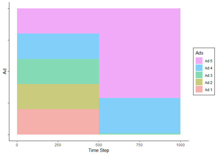
As expected, during the first 500 trials the ads were seen an even proportion of the time. In the next 500 trials, Ad 5 (the highest performer) was seen the most often, followed by Ad 4, and very rarely, Ad3.

In the next simulation, we can use the contextual package to look at an Epsilon Greedy algorithm with ε = 0.10. This means that it will explore randomly only 10% of the time, exploiting 90% of the time.

library(contextual)

# EPSILON GREEDY
horizon <- 1000L
simulations <- 1000L
conversionProbabilities <- c(0.05, 0.10, 0.15, 0.20, 0.25) 

bandit <- BasicBernoulliBandit$new(weights = conversionProbabilities)
policy <- EpsilonGreedyPolicy$new(epsilon = 0.10)
agent <- Agent$new(policy, bandit)

historyEG <- Simulator$new(agent, horizon, simulations)$run()

plot(historyEG, type = "arms", 
     legend_labels = c('Ad 1', 'Ad 2', 'Ad 3', 'Ad 4', 'Ad 5'),
     legend_title = 'Epsilon Greedy',
     legend_position = "topright",
     smooth = TRUE)

summary(historyEG)

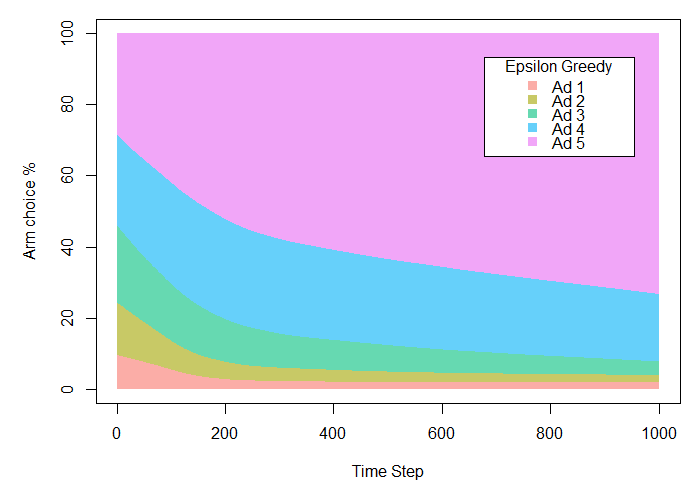
Here we can see that the Epsilon Greedy algorithm is quickly able to determine that Ad 5 is superior, improving over time. The total payoff is 217.11 conversions, or about 87% of the total possible payoff. This is also approximately 16% higher than with the A/B test, because the algorithm is able to begin exploiting the most successful ad much more quickly than with traditional methods.

Finally, we can compare both of these examples to Thompson Sampling, also using the contextual package.

# THOMPSON SAMPLING
horizon <- 1000L
simulations <- 1000L
conversionProbabilities <- c(0.05, 0.10, 0.15, 0.20, 0.25) 

bandit <- BasicBernoulliBandit$new(weights = conversionProbabilities)
policy <- ThompsonSamplingPolicy$new(alpha = 1, beta = 1)
agent <- Agent$new(policy, bandit)

historyThompson <- Simulator$new(agent, horizon, simulations)$run()

plot(historyThompson, type = "arms", 
     legend_labels = c('Ad 1', 'Ad 2', 'Ad 3', 'Ad 4', 'Ad 5'),
     legend_title = 'Thompson Sampling',
     legend_position = "topright",
     smooth = TRUE)

summary(historyThompson)

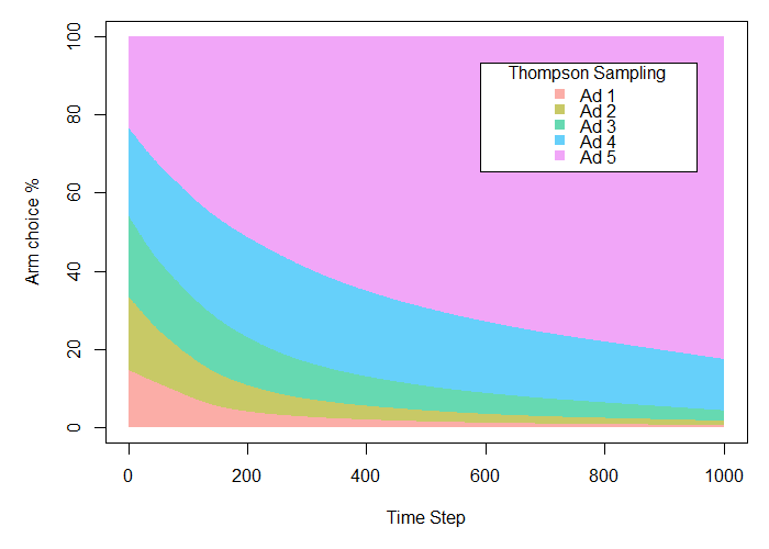
Thompson Sampling turns out to be our most successful model, resulting in a payoff of 219.97 (or almost 88% of the total conversions hypothetically achievable), over 17% more than with traditional A/B testing.

What’s more, while these results appear not too different from those in the Epsilon Greedy example, it is important to note that this would change with further trials. Since Epsilon Greedy is committed to exploring 10% of the time throughout the entire experiment, there is a limit to the extent that the algorithm can continue to optimize. Thompson Sampling is not similarly constrained, and rather can fully exploit the most successful option once it has been determined.

Overall, Bandit algorithms can provide an excellent solution for many use cases. In essence, they are a “light” form of reinforcement learning, where the algorithm auto-optimizes without knowledge of the task in advance, and earns rewards from the environment. Reinforcement learning, and its applications for online marketing, will be discussed in a future blog.