TabICL v2 for Time Series: A user test and benchmark comparison
Foundation models like TabICL v2 are increasingly finding their way into time series forecasting. But how does such a model perform against established methods like XGBoost or Meta’s Prophet? In this article, we summarize our findings and benchmark results.
Database & Feature Engineering
For our test, we use real-world data on nitrogen dioxide (NO2). The data was collected at hourly intervals at monitoring stations located near traffic roads. The data is characterized by strong daily and weekend patterns (traffic peaks) as well as seasonal differences (higher values in winter). There is no pronounced long-term trend.
Since TabICL and XGBoost do not process sequential time series structures natively, we equipped both models with similar feature engineering:
- Calendar features: Hour of the day, day of the week, etc.
- Lag features (past observations of the target variable): 24h, 48h, and 1-week lags.
- Exogenous features: Wind speed, wind direction, temperature, precipitation, and traffic volume.
Used only for TabICL:
- Seasonality encoding: Sine and cosine transformations to represent continuous periods as well as automatic detection via Fourier analysis.
In the TabICL code base for time series, calendar features and seasonality encodings are generated automatically.
It should also be noted that in a production application, exogenous features would first be forecasted themselves in order to be used as features. For our analysis, we use the actual realized values.
Compared Models & Benchmark Setup
As an evaluation metric, we use the Mean Absolute Scaled Error (MASE). A value greater than 1.0 means that the model performs worse than a naive in-sample baseline. The metric is also used, for example, in the well-known GIFT-Eval Benchmark for time series. In addition, we present the results for the standard Mean Absolute Error (MAE).
We average the MASE across 5 monitoring stations and all test folds of our rolling-window cross-validation (CV). For the CV, we proceed as follows:
- Determine the length of the training period n
- The first fold uses May 2, 2023, as the test period and the n observations before it as the training period
- Shift the test and training periods forward by one day
- Repeat this until 365 days are covered to obtain the train-test folds
The test folds of the CV thus cover a full year.
The following models were compared:
- XGBoost (with feature engineering, hyperparameters tuned via Optuna)
- TabICL (with feature engineering)
- TabICL minimal (without exogenous features and lags)
- Meta Prophet (Additive regression model, without exogenous features and lags)
- Seasonal Naive Baseline
Results Overview
| Metric | Station 010 | Station 018 | Station 027 | Station 032 | Station 042 | Overall |
|---|---|---|---|---|---|---|
| count | 26305 | 26305 | 26305 | 26305 | 26305 | 131525 |
| mean | 18.71 | 15.69 | 8.96 | 8.91 | 16.49 | 13.75 |
| std | 11.51 | 11.30 | 7.38 | 7.60 | 11.09 | 10.75 |
| mad | 8.83 | 8.43 | 5.22 | 5.59 | 8.22 | 8.01 |
| min | 1.00 | 1.00 | 0.00 | 0.00 | 0.00 | 0.00 |
| 25% | 10.00 | 8.00 | 4.00 | 4.00 | 9.00 | 6.00 |
| 50% | 16.00 | 13.00 | 7.00 | 7.00 | 13.00 | 11.00 |
| 75% | 24.00 | 20.00 | 11.00 | 12.00 | 21.00 | 18.00 |
| max | 112.00 | 104.00 | 75.00 | 87.00 | 118.00 | 118.00 |
Table 1: Statistics on the distribution of NO2 values per station and overall. Period 2021-05-02 to 2024-05-02. mad = Mean absolute deviation.
| Training Period | TabICL | XGBoost | TabICL minimal | Prophet | Seasonal Naive | Shortfall XGB vs. TabICL |
|---|---|---|---|---|---|---|
| 2 Jahre | 0.478 | 0.500 | 0.659 | 0.763 | 0.951 | +4,60% |
| 1 Jahr | 0.519 | 0.522 | 0.684 | 0.777 | 0.973 | +0,58% |
| 6 M | 0.571 | 0.587 | 0.728 | 0.847 | 1.017 | +2,80% |
| 3 M | 0.592 | 0.616 | 0.713 | 0.823 | 1.017 | +4,05% |
| 1,5 M | 0.616 | 0.646 | 0.719 | 0.832 | 1.021 | +4,87% |
Table 2: MASE for different models and training period lengths. Shown are the average MASE values across test folds for all stations.
| Training Period | TabICL | XGBoost | TabICL minimal | Prophet | Seasonal Naive | Shortfall XGB vs. TabICL |
|---|---|---|---|---|---|---|
| 2 Jahre | 3.874 | 4.052 | 5.356 | 6.180 | 7.307 | +4,60% |
| 1 Jahr | 4.113 | 4.151 | 5.433 | 6.143 | 7.307 | +0,92% |
| 6 M | 4.334 | 4.468 | 5.536 | 6.368 | 7.307 | +3,09% |
| 3 M | 4.433 | 4.626 | 5.369 | 6.194 | 7.307 | +4,35% |
| 1,5 M | 4.550 | 4.799 | 5.347 | 6.229 | 7.307 | +5,47% |
Table 3: MAE for different models and training period lengths. Analogous to Table 2. Shown are the average MAE values across test folds for all stations.
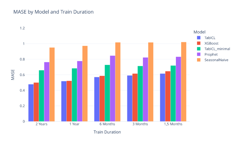 Figure 1: Bar plot comparing model MASE values across different training history lengths.
Discussion of Results
- Short histories (<= 6 months): With small data contexts, TabICL has an advantage. With 3 months of history, XGBoost is about 4% worse; with 1.5 months, it is nearly 5% worse.
- Medium history (1 year): With a one-year context, XGBoost and TabICL are virtually equal: XGBoost achieves a MASE of 0.522, while TabICL stands at 0.519.
- Full history (2 years): TabICL outperforms XGBoost by approx. 4.6% with a MASE of 0.478.
- TabICL out-of-the-box: Without manual feature engineering, TabICL significantly outperforms both Meta Prophet and the naive baseline.
- Second metric MAE: The Mean Absolute Error (MAE) confirms the results of the MASE.
- Size of the TabICL advantage: For the 2-year context, the MAE difference compared to XGBoost is around 0.18. This can be compared with the Mean Absolute Deviation (MAD) across all stations from Table 1. Put into proportion, this yields 0.18 / 8.01 = 0.02. The improvement is therefore 2% of how much the data fluctuates overall.
For one year of data and less, the pattern is clear: the less history available, the greater the advantage of TabICL. With 2 years of history, this trend breaks and TabICL's advantage increases again despite having more data. A likely explanation: TabICL can utilize the information from the extra year better than XGBoost to capture annual seasonality.
Forecast Stability: The standard deviation (SD) of the MAE across the 5 x 365 = 1,825 CV folds is approximately 2.5 for both XGBoost and TabICL. With an MAE of around 4, deviations of 6.5 units are to be expected, which is below the range of one standard deviation of the data (10.75, see Table 1).
In 57.5% of the folds, TabICL achieves the lower error. Thus, TabICL is better on average, but individual folds can still frequently be won by XGBoost.
Usability & Performance Insights
Integration of TabICL via the TabICLForecaster class and its predict_df method works well, but requires some familiarity. In the TabICL Repo, the prediction_length parameter is used. However, we find it clearer in practice to pass the future_df parameter alongside context_df, through which a pandas DataFrame can be provided. The future_df must contain a target column filled with NA values, a timestamp column with test observation timestamps, and, if used in context, the values of exogenous features.
Advantages
- The TabICLForecaster class automatically handles calendar features and seasonality transformations. As a result, TabICL can be applied immediately without custom feature engineering.
- TabICL v2 is open-source and can also be used for commercial projects free of charge (see license)
Disadvantages Regarding Hardware Requirements and Speed
- Speed: In our cross-validation (CV), TabICL was roughly 17 times slower than XGBoost when accounting for training time.
- Hardware requirements: On an NVIDIA L40S GPU, TabICL runs smoothly. On a modern laptop with CPU/GPU, a single CV run takes about 10x longer. On pure CPU, TabICL is currently hard to deploy practically.
- Inference: Because training and inference are blurred in in-context learning, higher runtimes per prediction occur. However, key-value caching offers potential to significantly reduce inference times in the future.
Conclusion: When to Use TabICL vs. XGBoost?
TabICL proves that tabular foundation models serve as excellent out-of-the-box baselines for time series. However, with proper feature engineering, the gap to XGBoost is small. Whether the gain in predictive performance is worth it should be evaluated based on practical relevance. Our general recommendations:
When TabICL is the right choice:
- Limited training data: For short training histories (< 3 to 6 months of hourly data, up to ~5K observations), TabICL delivers better results than XGBoost thanks to pre-training. But even with around 18K training observations, we see that TabICL can offer slight advantages.
- Quick baselines without domain knowledge: When little time is available for extensive feature engineering or hyperparameter tuning, TabICL delivers significantly better "out-of-the-box" results than Meta Prophet or naive baseline methods.
- Suitable hardware available: A powerful GPU is accessible.
- Small improvements have high leverage: In certain applications, even marginal improvements can scale to make a substantial impact.
When to use XGBoost:
- Very large datasets (> 60,000 observations): According to the developers, TabICL was not pre-trained for datasets exceeding 60K data points. XGBoost does not have this scaling restriction and seamlessly handles millions of rows.
- Constrained resources: When no GPU is available or the deployment infrastructure (e.g., edge devices) is memory-constrained.
- High speed requirements: TabICL is currently not suitable when inference and training times must be in the millisecond range, whereas XGBoost is.