Understanding and Handling Missing Data

Missing or incomplete data can have a huge negative impact on any data science project. This is particularly relevant for companies in the early stages of developing solid data collection and management systems.

While the best solution for missing data is to avoid it in the first place by developing good data-collection and stewardship policies, often we have to make due with what’s available.

This blog covers the different kinds of missing data, and what we can do about missing data once we know what we’re dealing with. These strategies range from simple - for example, choosing models that handle missings automatically, or simply deleting problematic observations - to (probably superior) methods for estimating what those missing values may be, otherwise known as imputation.

Types of Missing Data

Before we do anything to our data, we need to have a clear understanding of what kind of missingness is present. There are three main categories of missing data:

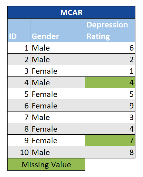
Missing Completely at Random (MCAR): In this scenario, the missing data are unrelated to the observation being studied or the other variables in the data set. Essentially, there are no systemic differences between the observations with and without missing data. This could be the case if, for example, individual survey-takers were only shown a selection of the total number of possible questions. With data that are MCAR, we can simply conduct our analyses on those observations with complete data. However, MCAR data are highly unusual in practice. A good rule of thumb is that if you can predict which units have missing data (with common sense, regression, etc.), then they are not MCAR.

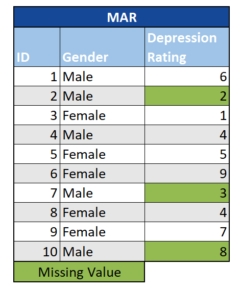
Missing at Random (MAR): In this case, the fact that data are missing can be predicted from the other variables in the study, but not from the missing data themselves. For example, say we know that men are less likely to answer survey questions on depression than women are. If the probability of an individual skipping a question on depression is only related to their gender (which we observe) but not their level of depression (which is unobserved), we can consider the data to be MAR. Depending on the analysis method employed, data sets with data that are MAR can be biased, and therefore missing data need to be considered early on in the process.

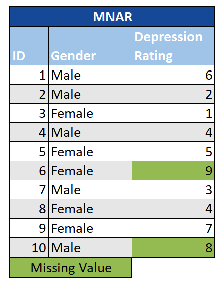
Missing Not at Random (MNAR): With data that are MNAR, the missingness is directly related to the value of the missing observation. Building on the example above, a survey question on depression would be MNAR if those with particularly high levels of depression refused to answer. This results in missing data that we cannot ignore or drop without introducing bias into our analysis - even imputing missing values may lead to misleading results. In severe cases, we may need to go back to the drawing board, and re-gather our data with an improved data-collection strategy.

Missing Data Solutions

Just Ignore It

While it may sound a bit silly, if you are confident that your data are MCAR, sometimes the easiest solution is simply to choose an algorithm that can automatically handle missing values. For example, XGBoost decides on the best imputation method for each sample without any extra steps being required.

Deletion

One potential way to handle missing values is to delete problematic observations or variables. This can happen in several ways:

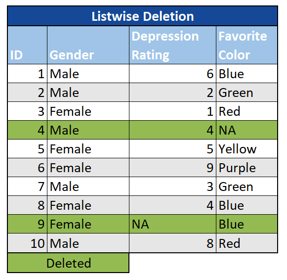
Listwise: In this scenario, an observation with a missing value in any variable would be removed entirely. Often referred to as “complete case analysis,” listwise-deletion is an easy solution if there are only a few observations with MCAR values among an otherwise large sample size. However, if the sample size is small or the data are not MCAR, listwise-deletion can introduce bias into the analysis.

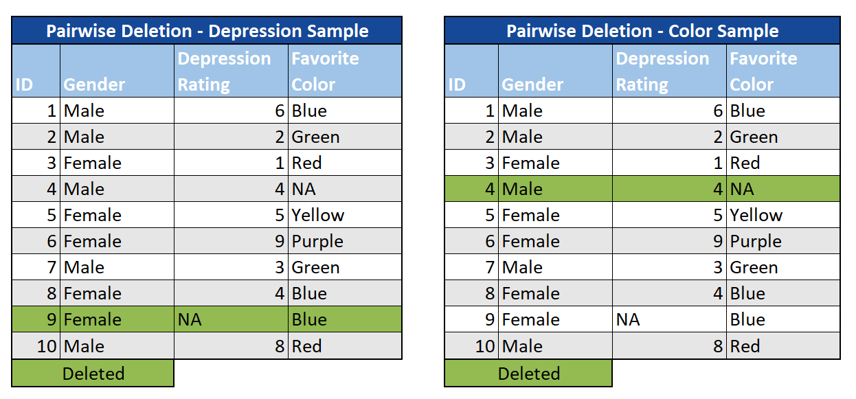
Pairwise: We can also choose to omit cases with MCAR data on the variables we are interested in, but not for other analyses. In this case, we look at subsets of the data that have complete cases, which preserves more information in comparison to listwise-deletion. However, since the samples are different throughout your study, interpretation becomes a challenge.

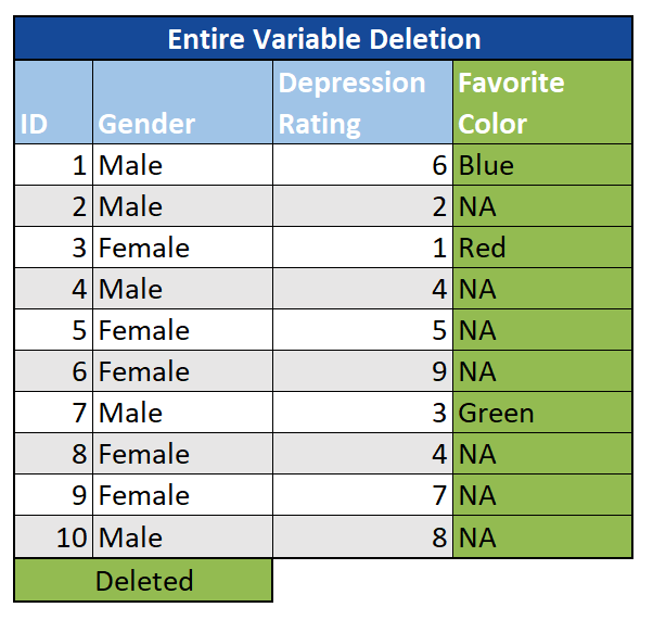
Entire variables: A final option is to omit an entire variable (column) from the analysis. While there is no rule of thumb for when this should happen, in situations where a large amount of data is missing (say, 60%+), and the variable is insignificant, simply excluding it may be an option if necessary.

Imputation

Imputation - or filling-in missing values according to some rule - is typically the best strategy for handling missing data. There are many ways to approach this, ranging from simple to complex. A few potential options are discussed below:

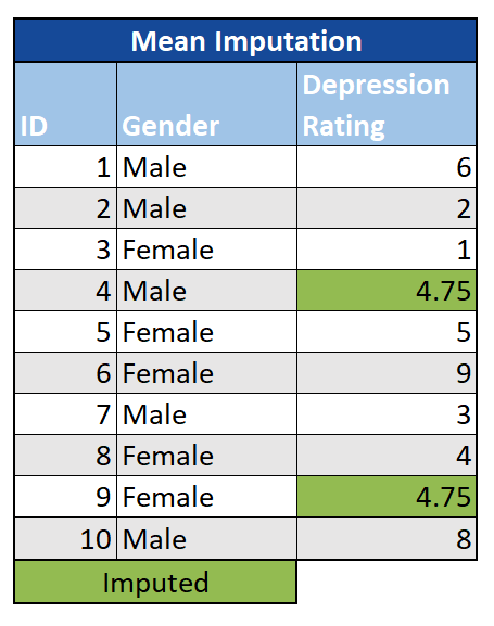
Mean/median/mode Simply using the mean or median in place of the missing value is a straight-forward method of imputation. This works by calculating the mean or median value in a particular column, and then replacing the missing data with this value. A similar approach for categorical data is to replace missings with the most common value (mode). This can be done either for the entire dataset, or a subset (for example, by first stratifying on age or gender and then imputing the mean for the appropriate subsample). Besides simplicity, a key advantage is that with mean imputation, the sample mean remains the same for the imputed data. We also know from sampling theory that using the mean as an assumed value makes sense, given that the mean is a reasonable estimate for randomly-selected observation with normally-distributed data. However, a key disadvantage is that it reduces variance in the data set and distorts the covariance among the remaining variables.

K Nearest Neighbors (KNN)
KNN imputes missing values by finding the k most similar observations (on the basis of some distance measure) and taking the mean/median/mode of those neighbors. This method requires determining the appropriate number of neighbors to consider, as well as how “distance” should best be measured. KNN works well for both continuous as well as categorical data, and its non-parametric nature can be very useful if the data follow an unusual pattern. A key drawback of the algorithm, however, is that it is quite computationally expensive, and is not well-suited to high-dimensional data where there is little difference between the closest neighbor and the furthest.

Linear Regression
Linear regression can be used to impute missing values by using the existing variables to make a prediction about the missing value. A disadvantage with this method is that because the imputed values are predicted by other variables, the standard errors are reduced. Additionally, it’s necessary to assume that there is a linear relationship between the variables in the data set, which may not be the case.

Last Observation Carried Forward (LOCF)/Next Observation Carried Backward (NOCB)
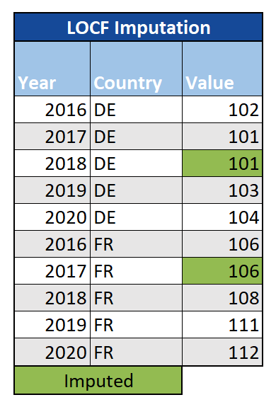
For time-series data, a straight-forward option is to use the last observed value for any missing data. Similarly, we could use the first observation after the missing value, which is referred to as Next Observation Carried Backward (NOCB). While these methods are easy to communicate and understand, they may not adequately account for fluctuations in the trend of the data over time.

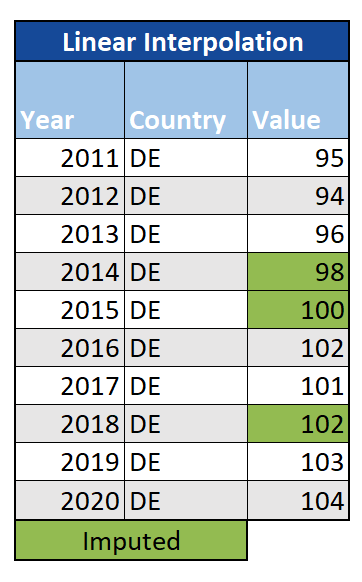
Linear Interpolation
Another option for time-series data is linear interpolation, where missing values are filled by considering the observations both before and after them (for example, by taking the mean value, or by evenly dividing the difference between the previous and next observations into as many missing values as need to be filled). While this may be an improvement on LOCF and NOCB, if the trend of the data is particularly complex it may not be sufficient, and it is not appropriate for seasonal data.

Multiple Imputation by Chained Equations (MICE)
With multiple imputation, the distribution of the observed data is taken into account, and several plausible estimates for the missing value are created. Multiple data sets are created and analyzed individually to obtain a set of parameter estimates. This method better accounts for uncertainty in the missing values, and is able to effectively handle continuous as well as categorical data.

This is not an exhaustive list, and many other imputation methods exist (such as imputation using random forests, GANs, etc.). There is no one-size-fits-all option that is always superior for handling missing data, but rather it is important to consider the nature of your data and the missing values to make an informed decision about how best to approach it.